


Reliability and resilience: expect failure and organise recovery
Design for failure before failure happens
Starting question — How do we keep a Mars system useful after something breaks?
Intuition. Reliability reduces the chance of failure; resilience assumes failures will still occur and designs detection, isolation, degraded operation, repair and recovery around that fact.
- Explain the governing idea before calculating.
- Name the units, evidence source and operational boundary of every key quantity.
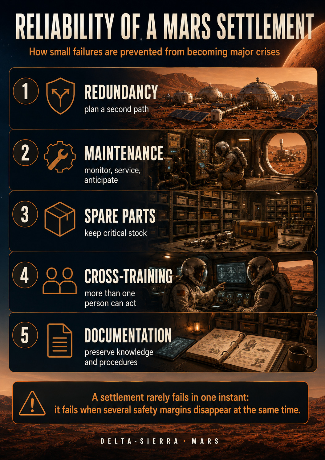


A Mars mission cannot honestly promise that no component will fail. It must instead show that credible faults can be detected, isolated well enough, tolerated in a degraded state and repaired with available resources. This module separates reliability, availability, redundancy, maintainability and resilience, then connects them through practical analysis methods.
Zero-prerequisite concepts
failure mode
Definition. A failure mode is a specific way a function can be lost, degraded, intermittent or latent.
Example. A pump can seize, leak, lose power or deliver insufficient flow; these are different failure modes with different detection and recovery paths.
Pitfall. Do not write only “pump fails”; that hides the mechanism and makes mitigation vague.
Ask what observable symptom distinguishes this failure mode from the others.
Guided exercise — failure mode
In a Mars mission scenario, identify one situation in which “failure mode” changes an engineering or operational decision. State the evidence you would inspect, the mistake you must avoid, and one independent check you would perform before accepting the decision.
Detailed correction — failure mode
Core meaning. A failure mode is a specific way a function can be lost, degraded, intermittent or latent.
Mission example. A pump can seize, leak, lose power or deliver insufficient flow; these are different failure modes with different detection and recovery paths.
Error to reject. Do not write only “pump fails”; that hides the mechanism and makes mitigation vague.
Independent check. Ask what observable symptom distinguishes this failure mode from the others.
- Quantification
- Use the physical unit that belongs to failure mode when it is quantitative; if it is qualitative, do not invent a numerical unit.
- Verification
- Compare the conclusion with the mission example, the stated pitfall and the mental check before using failure mode operationally.
redundancy
Definition. Redundancy provides more than one means of delivering a required function so that one loss does not immediately remove the service.
Example. Two independently powered pressure sensors can preserve a measurement after one sensor fails.
Pitfall. Two identical boxes fed by one breaker are not independent redundancy against breaker loss.
Trace power, software, connectors, environment and procedure before calling two channels independent.
Guided exercise — redundancy
In a Mars mission scenario, identify one situation in which “redundancy” changes an engineering or operational decision. State the evidence you would inspect, the mistake you must avoid, and one independent check you would perform before accepting the decision.
Detailed correction — redundancy
Core meaning. Redundancy provides more than one means of delivering a required function so that one loss does not immediately remove the service.
Mission example. Two independently powered pressure sensors can preserve a measurement after one sensor fails.
Error to reject. Two identical boxes fed by one breaker are not independent redundancy against breaker loss.
Independent check. Trace power, software, connectors, environment and procedure before calling two channels independent.
- Quantification
- Use the physical unit that belongs to redundancy when it is quantitative; if it is qualitative, do not invent a numerical unit.
- Verification
- Compare the conclusion with the mission example, the stated pitfall and the mental check before using redundancy operationally.
degraded mode
Definition. A degraded mode deliberately preserves the most important functions at reduced performance after a fault.
Example. A habitat may disable nonessential laboratory loads to preserve life support and communications.
Pitfall. Degraded mode is not uncontrolled deterioration; it is a defined, tested configuration.
Name which functions remain, which are shed and the criterion for leaving degraded mode.
Guided exercise — degraded mode
In a Mars mission scenario, identify one situation in which “degraded mode” changes an engineering or operational decision. State the evidence you would inspect, the mistake you must avoid, and one independent check you would perform before accepting the decision.
Detailed correction — degraded mode
Core meaning. A degraded mode deliberately preserves the most important functions at reduced performance after a fault.
Mission example. A habitat may disable nonessential laboratory loads to preserve life support and communications.
Error to reject. Degraded mode is not uncontrolled deterioration; it is a defined, tested configuration.
Independent check. Name which functions remain, which are shed and the criterion for leaving degraded mode.
- Quantification
- Use the physical unit that belongs to degraded mode when it is quantitative; if it is qualitative, do not invent a numerical unit.
- Verification
- Compare the conclusion with the mission example, the stated pitfall and the mental check before using degraded mode operationally.
resilience
Definition. Resilience is the ability to absorb a disruption, keep an acceptable mission function, reconfigure and recover.
Example. A rover with a failed wheel drive may adopt speed limits and a new route while maintenance is prepared.
Pitfall. High reliability alone does not prove resilience because even rare failures can still occur.
Imagine one plausible failure and trace detection, safe continuation, repair and return to normal service.
Guided exercise — resilience
In a Mars mission scenario, identify one situation in which “resilience” changes an engineering or operational decision. State the evidence you would inspect, the mistake you must avoid, and one independent check you would perform before accepting the decision.
Detailed correction — resilience
Core meaning. Resilience is the ability to absorb a disruption, keep an acceptable mission function, reconfigure and recover.
Mission example. A rover with a failed wheel drive may adopt speed limits and a new route while maintenance is prepared.
Error to reject. High reliability alone does not prove resilience because even rare failures can still occur.
Independent check. Imagine one plausible failure and trace detection, safe continuation, repair and return to normal service.
- Quantification
- Use the physical unit that belongs to resilience when it is quantitative; if it is qualitative, do not invent a numerical unit.
- Verification
- Compare the conclusion with the mission example, the stated pitfall and the mental check before using resilience operationally.
Calculation laboratory — formula, units, inverse check and limits
Quantitative mini-lessons
Reliability with a constant failure rate
- 1 — Concrete question
- What does “R = exp(−lambda×t)” compute in “Reliability with a constant failure rate”?
- 2 — Intuition without symbols
- When instantaneous risk stays constant, the probability of surviving declines progressively with time.
- 3 — Quantities
- R: probability of surviving without failure; lambda: constant failure rate; t: duration
- 4 — Formula
- R = exp(−lambda×t)
- 5 — Read aloud
- Read “R = exp(−lambda×t)” by naming every operation, subscript and grouping explicitly.
- 6 — Symbols and meaning
- R: probability of surviving without failure; lambda: constant failure rate; t: duration
- 7 — Pronunciation
- The “Read aloud” line above is the oral reference for “Reliability with a constant failure rate”. Any subscript, exponent or grouping that changes the meaning of the relation should be spoken explicitly.
- 8 — Units
- R dimensionless; lambda in 1/h; t in h
- 9 — Convention
- For “Reliability with a constant failure rate”, substitute values without changing the reference frame, time basis, system boundary or sign convention halfway through the calculation. Stated units: R dimensionless; lambda in 1/h; t in h.
- 10 — Why this operation
- The exponential law represents evolution proportional to the remaining state rather than a fixed linear decrement.
- 11 — Assumptions
- The rate parameter is assumed constant over the interval and events follow the stated model.
- 12 — Unit check
- R dimensionless; lambda in 1/h; t in h Verify that dimensional reduction reaches the unit of the requested output.
- 13 — Numerical case
- With lambda = 0.0005 1/h and t = 1,000 h, R = exp(−0.5) ≈ 0.6065.
- 14 — Why the calculation works
- The exponential law represents evolution proportional to the remaining state rather than a fixed linear decrement.
- 15 — Independent check
- Taking the natural logarithm of the result recovers the rate-times-duration product.
- 16 — Mental estimate
- A small rate-times-duration product gives a result near one; a large product moves it away rapidly.
- 17 — Interpretation
- This probability describes the selected model, not the certain future of a particular component.
- 18 — What the result does not prove
- For “Reliability with a constant failure rate”, the number obtained answers only the model “R = exp(−lambda×t)” under the stated scenario. It does not by itself validate the input data or the model outside those conditions.
- 19 — Sensitivity
- Time and rate combine through their product, then the exponential magnifies the change.
- 20 — Guided and autonomous exercises
Guided exercise. lambda = 0.0002 1/h and t = 500 h.
Detailed guided correction — open after trying
lambda = 0.0002 1/h and t = 500 h. R = exp(−0.10) ≈ 0.9048.
Autonomous exercise. lambda = 0.001 1/h and t = 200 h.
Autonomous correction — open after trying
lambda = 0.001 1/h and t = 200 h. R = exp(−0.20) ≈ 0.8187.
- 21 — Mission decision
- Use this law only when an approximately constant failure rate is defensible over the phase being studied.
Intrinsic availability
- 1 — Concrete question
- What does “A = MTBF / (MTBF + MTTR)” compute in “Intrinsic availability”?
- 2 — Intuition without symbols
- Availability improves when operating intervals are long and repairs are short.
- 3 — Quantities
- A: availability; MTBF: mean time between failures; MTTR: mean time to repair
- 4 — Formula
- A = MTBF / (MTBF + MTTR)
- 5 — Read aloud
- Read “A = MTBF / (MTBF + MTTR)” by naming every operation, subscript and grouping explicitly.
- 6 — Symbols and meaning
- A: availability; MTBF: mean time between failures; MTTR: mean time to repair
- 7 — Pronunciation
- The “Read aloud” line above is the oral reference for “Intrinsic availability”. Any subscript, exponent or grouping that changes the meaning of the relation should be spoken explicitly.
- 8 — Units
- A dimensionless; MTBF and MTTR in the same time unit
- 9 — Convention
- For “Intrinsic availability”, substitute values without changing the reference frame, time basis, system boundary or sign convention halfway through the calculation. Stated units: A dimensionless; MTBF and MTTR in the same time unit.
- 10 — Why this operation
- In “Intrinsic availability”, division relates a quantity to a reference, duration or capacity; the denominator must belong to the same case and remain non-zero.
- 11 — Assumptions
- The relation “A = MTBF / (MTBF + MTTR)” applies here only to the scenario described by the card. Inputs must be mutually consistent and satisfy the physical assumptions associated with “Intrinsic availability”.
- 12 — Unit check
- A dimensionless; MTBF and MTTR in the same time unit Verify that dimensional reduction reaches the unit of the requested output.
- 13 — Numerical case
- With MTBF = 1,000 h and MTTR = 10 h, A = 1,000/1,010 ≈ 0.9901, or 99.01%.
- 14 — Why the calculation works
- The numerical case applies “A = MTBF / (MTBF + MTTR)” directly to the stated values. The calculation is meaningful because the quantities are substituted into the same relation before the result is interpreted for “Intrinsic availability”.
- 15 — Independent check
- Quick check: multiplying the result by the denominator should reconstruct the numerator of “Intrinsic availability” within rounding.
- 16 — Mental estimate
- Before calculating “Intrinsic availability” precisely, round the inputs to one useful digit and predict the sign and order of magnitude. The detailed result should remain consistent with that estimate.
- 17 — Interpretation
- The formula directly shows why maintainability can partly compensate for a given failure frequency.
- 18 — What the result does not prove
- For “Intrinsic availability”, the number obtained answers only the model “A = MTBF / (MTBF + MTTR)” under the stated scenario. It does not by itself validate the input data or the model outside those conditions.
- 19 — Sensitivity
- Vary one input at a time around the nominal case to identify what drives the result of “Intrinsic availability” and whether that variation can change the mission decision.
- 20 — Guided and autonomous exercises
Guided exercise. MTBF = 500 h and MTTR = 5 h.
Detailed guided correction — open after trying
MTBF = 500 h and MTTR = 5 h. A = 500/505 ≈ 0.9901 = 99.01%.
Autonomous exercise. MTBF = 800 h and MTTR = 20 h.
Autonomous correction — open after trying
MTBF = 800 h and MTTR = 20 h. A = 800/820 ≈ 0.9756 = 97.56%.
- 21 — Mission decision
- Compare intrinsic with operational availability by accounting separately for logistic and administrative delay.
Reliability of a series chain
- 1 — Concrete question
- What does “R_series = R1×R2×R3” compute in “Reliability of a series chain”?
- 2 — Intuition without symbols
- In a chain where every item is required, all items must survive for the function to survive.
- 3 — Quantities
- R_series: chain reliability; R1: reliability of item one; R2: reliability of item two; R3: reliability of item three
- 4 — Formula
- R_series = R1×R2×R3
- 5 — Read aloud
- Read “R_series = R1×R2×R3” by naming every operation, subscript and grouping explicitly.
- 6 — Symbols and meaning
- R_series: chain reliability; R1: reliability of item one; R2: reliability of item two; R3: reliability of item three
- 7 — Pronunciation
- The “Read aloud” line above is the oral reference for “Reliability of a series chain”. Any subscript, exponent or grouping that changes the meaning of the relation should be spoken explicitly.
- 8 — Units
- all reliability terms dimensionless
- 9 — Convention
- For “Reliability of a series chain”, substitute values without changing the reference frame, time basis, system boundary or sign convention halfway through the calculation. Stated units: all reliability terms dimensionless.
- 10 — Why this operation
- In “Reliability of a series chain”, multiplication combines the factors that directly build the requested quantity; the factors must describe the same case.
- 11 — Assumptions
- The relation “R_series = R1×R2×R3” applies here only to the scenario described by the card. Inputs must be mutually consistent and satisfy the physical assumptions associated with “Reliability of a series chain”.
- 12 — Unit check
- all reliability terms dimensionless Verify that dimensional reduction reaches the unit of the requested output.
- 13 — Numerical case
- With R1 = 0.99, R2 = 0.98 and R3 = 0.97, R_series = 0.99×0.98×0.97 ≈ 0.9411.
- 14 — Why the calculation works
- The numerical case applies “R_series = R1×R2×R3” directly to the stated values. The calculation is meaningful because the quantities are substituted into the same relation before the result is interpreted for “Reliability of a series chain”.
- 15 — Independent check
- Quick check: for any non-zero factor, dividing the result by that factor should recover the other expected contribution in “Reliability of a series chain”.
- 16 — Mental estimate
- Before calculating “Reliability of a series chain” precisely, round the inputs to one useful digit and predict the sign and order of magnitude. The detailed result should remain consistent with that estimate.
- 17 — Interpretation
- Even very good components can form a substantially less reliable chain when every one is mandatory.
- 18 — What the result does not prove
- For “Reliability of a series chain”, the number obtained answers only the model “R_series = R1×R2×R3” under the stated scenario. It does not by itself validate the input data or the model outside those conditions.
- 19 — Sensitivity
- Vary one input at a time around the nominal case to identify what drives the result of “Reliability of a series chain” and whether that variation can change the mission decision.
- 20 — Guided and autonomous exercises
Guided exercise. R1 = 0.995, R2 = 0.990, R3 = 0.985.
Detailed guided correction — open after trying
R1 = 0.995, R2 = 0.990, R3 = 0.985. R_series ≈ 0.9703.
Autonomous exercise. R1 = R2 = R3 = 0.95.
Autonomous correction — open after trying
R1 = R2 = R3 = 0.95. R_series = 0.95³ ≈ 0.8574.
- 21 — Mission decision
- Identify components that are truly in series before multiplying probabilities.
Two-unit independent redundancy
- 1 — Concrete question
- What does “R_parallel = 1 − (1 − R_unit)^2” compute in “Two-unit independent redundancy”?
- 2 — Intuition without symbols
- Two independent units let the function survive as long as at least one remains available.
- 3 — Quantities
- R_parallel: redundant-function reliability; R_unit: reliability of one identical unit
- 4 — Formula
- R_parallel = 1 − (1 − R_unit)^2
- 5 — Read aloud
- Read “R_parallel = 1 − (1 − R_unit)^2” by naming every operation, subscript and grouping explicitly.
- 6 — Symbols and meaning
- R_parallel: redundant-function reliability; R_unit: reliability of one identical unit
- 7 — Pronunciation
- The “Read aloud” line above is the oral reference for “Two-unit independent redundancy”. Any subscript, exponent or grouping that changes the meaning of the relation should be spoken explicitly.
- 8 — Units
- reliability terms dimensionless
- 9 — Convention
- For “Two-unit independent redundancy”, substitute values without changing the reference frame, time basis, system boundary or sign convention halfway through the calculation. Stated units: reliability terms dimensionless.
- 10 — Why this operation
- In “Two-unit independent redundancy”, subtraction measures a margin or difference between comparable quantities expressed in the same frame.
- 11 — Assumptions
- The relation “R_parallel = 1 − (1 − R_unit)^2” applies here only to the scenario described by the card. Inputs must be mutually consistent and satisfy the physical assumptions associated with “Two-unit independent redundancy”.
- 12 — Unit check
- reliability terms dimensionless Verify that dimensional reduction reaches the unit of the requested output.
- 13 — Numerical case
- With R_unit = 0.90, R_parallel = 1 − 0.10² = 0.99.
- 14 — Why the calculation works
- The numerical case applies “R_parallel = 1 − (1 − R_unit)^2” directly to the stated values. The calculation is meaningful because the quantities are substituted into the same relation before the result is interpreted for “Two-unit independent redundancy”.
- 15 — Independent check
- Quick check: adding the subtracted term back to the result should reconstruct the starting quantity in “Two-unit independent redundancy”.
- 16 — Mental estimate
- Before calculating “Two-unit independent redundancy” precisely, round the inputs to one useful digit and predict the sign and order of magnitude. The detailed result should remain consistent with that estimate.
- 17 — Interpretation
- The gain disappears if a common cause can disable both units together.
- 18 — What the result does not prove
- For “Two-unit independent redundancy”, the number obtained answers only the model “R_parallel = 1 − (1 − R_unit)^2” under the stated scenario. It does not by itself validate the input data or the model outside those conditions.
- 19 — Sensitivity
- Vary one input at a time around the nominal case to identify what drives the result of “Two-unit independent redundancy” and whether that variation can change the mission decision.
- 20 — Guided and autonomous exercises
Guided exercise. R_unit = 0.95.
Detailed guided correction — open after trying
R_unit = 0.95. R_parallel = 1 − 0.05² = 0.9975.
Autonomous exercise. R_unit = 0.80.
Autonomous correction — open after trying
R_unit = 0.80. R_parallel = 1 − 0.20² = 0.96.
- 21 — Mission decision
- Validate physical, functional and procedural independence before crediting redundancy gain.
Remaining capacity after a loss
- 1 — Concrete question
- What does “C_remaining = C_nominal − C_lost” compute in “Remaining capacity after a loss”?
- 2 — Intuition without symbols
- Operational resilience is often measured by service that remains after a failure, not merely by the existence of the failure.
- 3 — Quantities
- C_remaining: still-usable capacity; C_nominal: nominal capacity; C_lost: lost or unavailable capacity
- 4 — Formula
- C_remaining = C_nominal − C_lost
- 5 — Read aloud
- Read “C_remaining = C_nominal − C_lost” by naming every operation, subscript and grouping explicitly.
- 6 — Symbols and meaning
- C_remaining: still-usable capacity; C_nominal: nominal capacity; C_lost: lost or unavailable capacity
- 7 — Pronunciation
- The “Read aloud” line above is the oral reference for “Remaining capacity after a loss”. Any subscript, exponent or grouping that changes the meaning of the relation should be spoken explicitly.
- 8 — Units
- all three capacities in the same operational unit
- 9 — Convention
- For “Remaining capacity after a loss”, substitute values without changing the reference frame, time basis, system boundary or sign convention halfway through the calculation. Stated units: all three capacities in the same operational unit.
- 10 — Why this operation
- In “Remaining capacity after a loss”, subtraction measures a margin or difference between comparable quantities expressed in the same frame.
- 11 — Assumptions
- The relation “C_remaining = C_nominal − C_lost” applies here only to the scenario described by the card. Inputs must be mutually consistent and satisfy the physical assumptions associated with “Remaining capacity after a loss”.
- 12 — Unit check
- all three capacities in the same operational unit Verify that dimensional reduction reaches the unit of the requested output.
- 13 — Numerical case
- With C_nominal = 12 units/h and C_lost = 4 units/h, C_remaining = 8 units/h.
- 14 — Why the calculation works
- The numerical case applies “C_remaining = C_nominal − C_lost” directly to the stated values. The calculation is meaningful because the quantities are substituted into the same relation before the result is interpreted for “Remaining capacity after a loss”.
- 15 — Independent check
- Quick check: adding the subtracted term back to the result should reconstruct the starting quantity in “Remaining capacity after a loss”.
- 16 — Mental estimate
- Before calculating “Remaining capacity after a loss” precisely, round the inputs to one useful digit and predict the sign and order of magnitude. The detailed result should remain consistent with that estimate.
- 17 — Interpretation
- This remaining margin must be compared with the minimum requirement of the degraded mode.
- 18 — What the result does not prove
- For “Remaining capacity after a loss”, the number obtained answers only the model “C_remaining = C_nominal − C_lost” under the stated scenario. It does not by itself validate the input data or the model outside those conditions.
- 19 — Sensitivity
- Vary one input at a time around the nominal case to identify what drives the result of “Remaining capacity after a loss” and whether that variation can change the mission decision.
- 20 — Guided and autonomous exercises
Guided exercise. C_nominal = 20 kW and C_lost = 6 kW.
Detailed guided correction — open after trying
C_nominal = 20 kW and C_lost = 6 kW. C_remaining = 20 − 6 = 14 kW.
Autonomous exercise. C_nominal = 50 L/h and C_lost = 15 L/h.
Autonomous correction — open after trying
C_nominal = 50 L/h and C_lost = 15 L/h. C_remaining = 50 − 15 = 35 L/h.
- 21 — Mission decision
- Enter safe mode if remaining capacity no longer covers the minimum vital function.
1. Reliability, availability and resilience ask different questions
Reliability concerns successful function over stated time and conditions. Availability also reflects restoration after failure. Resilience asks whether an acceptable mission can continue through disturbance, degradation and recovery. A system may fail often yet be quickly repairable, or fail rarely but catastrophically.
Reliability is the probability that an item performs its required function for a stated time under stated conditions. Availability asks whether the function is ready when demanded, so repair time also matters. Resilience goes further: can the system preserve an essential service, reconfigure and then return toward a sustainable state after the event? A highly reliable component can still create poor resilience if its rare failure is unrecoverable. Conversely, a component that fails more often may deliver excellent service if detection is fast, access is easy and degraded operation is acceptable. These three terms therefore need separate requirements and separate evidence.
2. MTBF is not a component death clock
MTBF is Mean Time Between Failures, a population statistic under defined use. In a simple exponential model, constant failure rate λ gives R(t)=e−λt. The model ignores infant mortality and wear-out; its assumptions must be stated.
MTBF, mean time between failures, is a population or model statistic, not the predicted death time of one component. Under a simplified exponential model with constant failure rate λ, reliability is R(t)=e^(−λt) and MTBF=1/λ. An MTBF of 10,000 hours does not mean the item will work for 10,000 hours and then fail. It describes an event rate assumed for a population. On Mars, a constant-rate model may be poor when wear, radiation, dust or thermal cycling dominate. The number should always be accompanied by the test environment, population, confidence and mechanisms that the model does not represent.
3. Availability exposes repair time
A simple intrinsic model is A = MTBF/(MTBF+MTTR), where MTTR is Mean Time To Repair. With MTBF 1,000 h and MTTR 10 h, availability is about 0.990. Reducing repair time increases availability without changing failure rate.
A common intrinsic-availability approximation is A = MTBF/(MTBF + MTTR). With MTBF = 1,000 h and MTTR = 10 h, A ≈ 1,000/1,010 = 0.990, or 99.0%. Reducing MTTR to 2 h raises it to about 99.8% without changing failure frequency. The calculation shows why access, diagnostics, tools and post-repair testability can matter as much as component reliability. But the formula assumes repair is possible and does not automatically include spare logistics, EVA waiting time, common-cause events or maintenance queues. Engineers must know what an availability number leaves out.
4. FMEA and FMECA walk through failure modes
A Failure Modes and Effects Analysis asks how a function can fail, its local and system effects, and how the failure is detected. FMECA adds criticality assessment. The value is the disciplined search for single failures, critical items and missing detection or maintenance provisions.
FMEA walks through functions or components and asks how each can fail, what the local and system effects are, how the failure is detected and what action limits the consequence. FMECA adds criticality. The value is not the spreadsheet itself but the discovery of hidden interfaces and uncovered modes. A row labelled ‘bad sensor’ should state whether the fault is detectable, whether software can believe it and which actuator could then be commanded incorrectly. For a Mars habitat, FMEA also needs maintenance, software, human action and post-repair states; otherwise it describes only pristine hardware rather than the system that will exist after years of operation.
5. Fault trees start from the unwanted event
Fault Tree Analysis begins with an event such as loss of pressure and works backward through combinations that can cause it. AND and OR logic can structure the argument, but the physical dependencies still matter. Drawing two branches separately does not prove statistical independence.

A fault tree starts from an unwanted top event and works backward to combinations of causes. An OR gate means any one cause is sufficient; an AND gate requires a combination. This is especially useful for exposing common causes. Two pumps may look redundant, but if loss of one shared power feed is enough to lose flow, the common branch dominates the tree. Probabilities can be added when independence assumptions are credible, but the primary value is logical: showing which combinations actually remove the service and where physical, electrical or software separation changes the outcome.
6. Redundancy only works when causes are sufficiently independent
Two pumps on one bus, two computers carrying the same software defect or two sensors exposed to the same contamination can fail together. Review power, cooling, code, connectors, calibration, environment and operator procedure for common paths.
Redundancy only helps when paths are sufficiently independent. Two computers in one enclosure may share power, temperature, connector, software and configuration error. One common event can therefore remove both. Diversity may be introduced through hardware, software, sensing principle or physical location, but it creates its own verification and maintenance cost. The review question is not ‘how many units?’ but ‘which causes can still remove them together?’ For a settlement, repairability also matters: two non-repairable units may be less resilient than one robust unit supported by replaceable modules, test equipment and a bypass.
7. FDIR means detection, isolation and recovery
Detection recognises abnormal evidence. Isolation narrows the likely fault. Recovery chooses a safe or degraded configuration. Required reaction time varies: a slow leak permits analysis; loss of attitude control may demand automatic action in seconds.
FDIR means Fault Detection, Isolation and Recovery: recognise that behaviour has left the expected domain, isolate the cause or at least the affected zone, and recover a safe function. Each step can fail. A threshold that is too sensitive creates false alarms; isolation that is too aggressive can disconnect the healthy channel; automatic recovery can reintroduce the fault. Evidence should therefore be graded. One threshold may request independent confirmation, a second enter a degraded mode, and later verification may permit return to service. The objective is not to automate every decision but to keep the state understandable and controllable throughout the anomaly.
8. Safe mode is a stable survival configuration
Safe mode preserves the functions that prevent further deterioration: power, thermal control, attitude, communications and sometimes life support. It must remain viable long enough to diagnose and repair. A “safe” state that drains a finite resource too quickly is only a short transient.
Safe mode is a stable configuration designed to preserve resources and prevent escalation. It does not mean ‘turn everything off’. A spacecraft must still generate power, control critical temperatures, maintain an attitude compatible with arrays and communications, and protect the crew. Safe mode therefore has its own power, sensing, actuation and duration requirements. If it depends on the component that just failed, it is not a genuine refuge. Validation injects faults and checks that the system can reach this state with the resources actually left, then confirms that a path exists for diagnosis and recovery.
9. Maintainability lives in physical access and testability
Isolation valves, test points, modular connectors and access can reduce restoration time dramatically. A supposedly redundant box that requires two days of disassembly may still create unacceptable downtime.
Maintainability is designed before failure. Access time, panel mass, connectors, working volume, tools, test points, electrical isolation and EVA requirements can dominate MTTR. A component that is easy to replace on a bench may be almost unreachable once installed behind two fluid lines. Design reviews should therefore rehearse the intervention with representative tools and constraints, then include reconfiguration and verification time. On Mars, a locally repaired item can also create a new configuration that must be recorded. Resilience depends on proving return to service, not merely on completing the mechanical replacement.
10. Failure scenario: recovery creates a new common dependency
A first failure causes two services to be transferred onto the same backup bus. A later backup-bus failure now removes both. The common cause was created by reconfiguration. Resilience analysis therefore needs degraded configurations as well as the nominal architecture.
Two independent failures can become a common failure through procedure. If the crew loads the same bad configuration file into two replacement controllers, hardware duplication no longer protects the function. An ambiguous checklist can likewise lead two operators to isolate the wrong valve. Human and organisational reliability therefore belong in system analysis. Critical procedures need observable criteria, independent confirmation for irreversible actions where practical, and controlled version management. Lessons learned should update the authoritative document without erasing history so that a corrected error does not reappear months later on another system.
Guided case — two pump architectures
Architecture A has two identical pumps in parallel; Architecture B has one operating pump, a manual bypass that preserves 60 percent flow and three easily replaceable modules. At first glance A looks more redundant. But if both A pumps share one controller and one power feed, a common cause can remove both. B may preserve 60 percent of service for eight hours, long enough to replace a module in two hours and verify it before full return.
Availability arithmetic alone is not enough. The sequence must include detection, stabilisation, access, physical repair, test and restart. A quoted 30-minute bench MTTR can become four hours in the habitat if access requires depressurising a zone or moving equipment.
The final exercise asks which change buys the most resilience: a third identical pump, a second power feed, a manual bypass, independent diagnostics or better access. The answer depends on the dominant cause revealed by the fault tree, not on raw component count.
11. Mini-project: build a resilience case
- Select a vital function.
- Define its top unwanted event.
- List five failure modes.
- Identify common causes.
- Describe detection, degraded service and repair.
- Calculate one simple availability metric.
- Add a second fault during degraded operation.
The case is useful when a reader can see what remains possible after failure and how full service returns.
12. Mission lab — compare redundancy with repairability
Consider two teaching architectures. Architecture A has two identical non-repairable pumps, either capable of full flow. Architecture B has one operating pump, three easily replaceable modules and a manual bypass. Which is “more reliable”? The question is incomplete. We need failure mechanisms, common causes, replacement time, spare inventory, allowable downtime and bypass capability.
If a module replacement takes two hours and bypass preserves 60 percent flow for eight hours, B may be highly resilient despite less instantaneous duplication. Conversely, if both pumps in A share one controller, their apparent redundancy does not protect against that common cause. Resilience is evaluated across the whole event sequence rather than from a block count.
Operational restoration time should separate detection time, stabilisation time, physical repair, test and return-to-service. A quoted MTTR based only on hands-on wrench time can be dangerously optimistic for Mars, where depressurisation, suit preparation or access may dominate the event.
The same idea applies to software. A hot spare computer that boots the same corrupted configuration may restore hardware but not function. Recovery evidence must prove the service, not merely that a redundant unit powered on.
13. Probability has limits; physical evidence still matters
A highly precise probability can look authoritative even when its input data is weak. Terrestrial populations may not represent Mars dust, radiation, partial gravity, multi-year isolation or the actual maintenance regime. Reliability models should therefore be paired with mechanism understanding, environmental test, inspection and operational evidence.
A reliability number is useful when it changes a decision: separate a common dependency, improve access, increase a spare quantity, alter an inspection interval or create a degraded mode. If the number has no design or operational consequence, it may be a dashboard decoration rather than engineering evidence.
For every critical probability, ask what event population created it, whether conditions match the mission, what confidence interval or uncertainty exists and which failure mechanisms are excluded. When evidence is sparse, bounding cases can be more honest than false precision.
Mission reasoning laboratory — connect the calculation to a real decision
Separate failure probability from mission consequence
Reliability analysis starts by asking how often something may fail, but mission design must also ask what happens next. A component with a modest failure rate can be tolerable when it is easy to detect, isolate and replace. A very reliable component can still dominate risk when one hidden failure removes the only oxygen-production train. For each critical function, list the failure mechanisms, observable symptoms, time available before harm, alternative paths and repair resources. That sequence turns a statistical number into an operational resilience argument.
Build redundancy around independent resources
Redundancy has value only when the channels do not share the same vulnerable cause. On Mars, common causes include a single power bus, one cooling loop, shared software, a common connector, dust exposure, a maintenance error or a procedure that commands both channels incorrectly. Draw the dependency chain behind each redundant unit. If two compressors share one upstream valve, or two computers share one corrupted data source, the apparent “two of everything” architecture may still behave like one system when the wrong event occurs.
Design detection before recovery
A recovery action cannot be trusted until the fault is detected and isolated with enough confidence. Detection should use observables that change early enough to preserve response time: current, pressure, temperature, flow, timing, position disagreement or self-test status. Isolation then asks which component or path is responsible. A false isolation can be worse than the original fault because it may switch off the healthy channel. Recovery logic therefore needs evidence thresholds, timeout behaviour and a safe fallback when diagnosis remains ambiguous.
Treat safe mode as a survival architecture
Safe mode is not “turn everything off.” Life support, thermal control, command reception, attitude or communications may need to remain active. The correct safe state depends on the vehicle and failure. A Mars habitat losing a high-power experiment may shed science loads while preserving air circulation, thermal control and emergency communications. A spacecraft with an attitude fault may point for power-positive survival rather than for science. Define the safe configuration by the minimum functions needed to preserve time and options for recovery.
Make repairability physical
Maintainability is constrained by human reach, fastener access, contamination control, tools, suit gloves, spare volume and the ability to verify a repair. A line-replaceable unit that requires removing ten unrelated panels is not genuinely maintainable during an emergency. Design fault isolation points, quick-disconnects and lifting aids before hardware is frozen. Mars adds communication delay and a long resupply interval, so a repair case should specify the spare, procedure, crew skill, expected time, isolation boundary and proof that the restored function is actually healthy.
Use degraded modes deliberately
A resilient colony does not need every function at full performance after every fault. It needs a controlled path that preserves survival and recovery. Examples include reducing crop lighting to protect battery reserve, parking one rover so its parts remain available for another, or limiting water-processing throughput while a redundant pump is serviced. Each degraded mode should state entry criteria, permitted duration, prohibited activities, resource implications and exit evidence. Without those boundaries, “operate degraded” becomes an excuse for accumulating hidden risk.
Close the resilience case with evidence
A credible resilience case combines analysis, test and operating experience. Fault-injection tests can show whether detection thresholds work. Maintenance demonstrations can show whether crew access and tools are adequate. Simulations can explore combinations that would be too destructive to test physically. The evidence record should also capture known gaps: untested common causes, uncertain repair time or hardware whose actual Martian dust behaviour remains unknown. Resilience is not a slogan attached to a block diagram; it is an argument whose assumptions can be audited and updated.
Progressive exercises — solve first, then open the correction
Exercise A — availability
A repairable unit has MTBF = 500 h and MTTR = 5 h. Using A = MTBF/(MTBF+MTTR), calculate steady-state availability and express it as a percentage. Then state one reason why this number alone does not prove mission resilience.
Detailed correction — Exercise A — availability
Calculation. A = 500/(500+5) = 500/505 ≈ 0.9901, or about 99.0%.
Interpretation. High availability says the unit is expected to be available most of the time under the assumed failure/repair model. It does not show whether failures are common-cause, whether repair resources exist on Mars, or whether the system can remain safe during the repair interval.
Exercise B — common cause
Two identical flight computers have separate power converters but run the same software build and receive the same corrupted navigation message. Explain whether the architecture is independent against this scenario, identify the common cause, and propose one mitigation that adds genuine diversity.
Detailed correction — Exercise B — common cause
Diagnosis. The computers are not independent against a shared software or data-input defect. Separate power does not remove a common software build or a common corrupted input.
Mitigation example. Add a dissimilar monitoring path, independent validation of critical navigation messages, or a separate safe-mode computer with constrained functions and separately verified software.
Beginner vocabulary checkpoint
- MTBF — Mean time between failures; a statistical reliability metric for repairable items, not a countdown timer.
- MTTR — Mean time to repair or restore; it includes the repair boundary defined by the analysis.
- availability — Fraction of time a required function is expected to be available under the stated failure and repair assumptions.
- FMEA — Failure Modes and Effects Analysis: a structured review of how elements can fail and what each failure does.
- FMECA — FMEA extended with criticality assessment so that failure consequences can be prioritised.
- fault tree — Top-down logic model that starts from an unwanted event and traces combinations of causes.
- FDIR — Fault Detection, Isolation and Recovery: the chain that identifies a fault, localises it and restores acceptable operation.
- safe mode — A predefined stable configuration intended to preserve essential survival and recovery capability after an anomaly.
- common-cause failure — One cause that defeats multiple supposedly redundant channels at the same time.
- latent failure — A failure that exists but is not immediately observable during normal operation.
- single-point failure — One failure whose occurrence can remove a required function without an independent recovery path.
- graceful degradation — Designed reduction in capability that preserves essential service instead of collapsing abruptly.
- maintainability — How readily a system can be inspected, accessed, diagnosed, repaired and returned to service.
- fault containment — Architecture that prevents a local fault from propagating into other functions or channels.
- cross-strapping — Connections that allow sources, loads or processing channels to be reconfigured across redundant paths.
- dispatch reliability — Probability or fraction of planned missions that can start without cancellation caused by technical unavailability.
- repair resource — Tool, spare, material, documentation, access or trained labour required to restore a failed function.
- proof test — Deliberate test used to reveal hidden failures that normal operation may not expose.
- degraded operation — Continued service with reduced capability under an approved post-fault configuration.
Sources and references
Verified primary supplement: NASA Systems Engineering Handbook
Engineering studio — compare two availability architectures
For a simple exponential model with no repair during the interval, reliability is R(t)=exp(−t/MTBF). With MTBF = 1,500 h and t = 500 h, R ≈ exp(−1/3) ≈ 0.716. Two genuinely independent parallel channels would then give a theoretical probability of retaining at least one channel of 1−(1−R)² ≈ 0.919. The exercise shows both the benefit of redundancy and how strongly it depends on the independence assumption.
The final trap is a common cause: both redundant channels share one power supply. The student explains why two identical units no longer provide true redundancy if a single failure can remove them together, proposes an architectural change — electrical separation, diversity or functional refuge — and defines the test that demonstrates the common cause has actually been broken.
The reliability exercise finally distinguishes repairability from diagnosability. A component may be physically replaceable yet operationally unavailable if the crew cannot identify the failed item with sufficient confidence. The student therefore assigns diagnostic evidence, access time and post-repair test criteria to each critical replacement, then checks whether common test equipment itself becomes a single point of failure.